Connectivity and quality¶

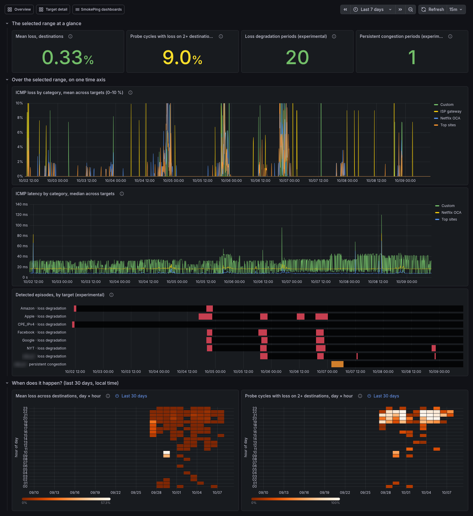
The Connectivity & Quality dashboard answers "is the connection's quality changing, and when?". The Overview tells you how things are right now. This dashboard puts the selected range (seven days by default) on one time axis, so a burst of loss, a step in latency and a detected episode line up vertically. Below that, it shows the last 30 days by hour of day, where a daily pattern stands out.

The Connectivity & Quality dashboard over seven days

Open it from the dashboard list (SmokePing dashboards) or from the Overview's Where to look next list. It is part of the InfluxDB dashboard set: Pro with ClickHouse does not have it.

The Service category variable at the top narrows the destinations to the targets in one or more service categories (video, gaming, ai_assistant...; see Service taxonomy). All, the default, counts every destination, labeled or not. The lines stay grouped by probe bucket; the whole-connection rows are not narrowed. How many targets of each category the Pi measures is on Targets by service, linked from this dashboard's header.

At a glance¶

Tile	What it counts
Mean loss, destinations	Share of pings lost across every destination over the range
Probe cycles with loss on 2+ destinations	Share of 5-minute cycles in which at least two destinations lost packets at once
Loss degradation periods	Periods the inference module found on destinations that overlap the range, when it is on
Persistent congestion periods	Periods Jitterbug labeled congested on destinations that overlap the range, when it is on

"Destinations" leaves out two kinds of target. The ISP gateway rate-limits ICMP and has a loss floor of its own. The DNS wizard's targets are left out because many CDNs drop ICMP. Both are ICMP targets like the rest, but counting them would make the numbers describe the probes rather than the connection.

The second tile is usually the more telling one. One destination losing packets is that destination's problem. Two or more losing in the same cycle point at something they share: the house, the line or the ISP. A cycle here is a 5-minute window, the default probe step. With a different frequency, the share is still comparable from one day to the next, but it is not a count of probe rounds.

On one time axis¶

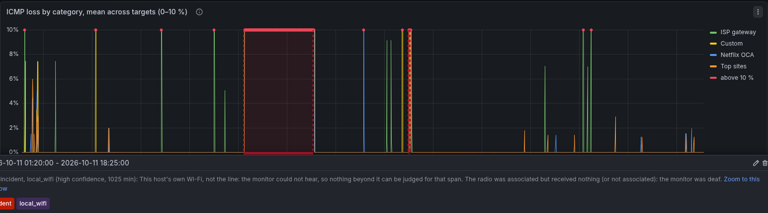
ICMP loss by category (0–10 %). This is the Overview's loss panel zoomed to the range where everyday loss lives. A cut above 10 % runs off the top; a red dot on the top edge marks each window where a category did, and the tooltip still shows the real value (the Overview shows the full scale). Several categories rising together is the link; one alone is its destinations. Unlike the tiles, this chart keeps the ISP gateway's line: it sits on its own floor, and a band the gateway does not share is beyond the access link.
ICMP latency by category. The median of the targets' medians, per kind of destination. The ISP gateway is left out: it answers ICMP from its control plane, whose spikes of hundreds of milliseconds would flatten every other line. The Overview's Toward the ISP panel charts it.
Detected episodes, by target (experimental). What the inference module found: red is loss degradation, orange is persistent congestion. Every target the module analyzes has a row, the ISP gateway included, so you can see whether the first hop moved too. These are detections, not confirmations. Compare them with the two panels above before believing one. Click a bar for every layer of that target over the same range, with the period shaded. The panel is empty unless the module is on (sudo smoking-pi enable inference).
Loss incidents (diagnosed). The dark red markers along the bottom of the charts are the alerter's diagnosed incidents (see alerting), whatever they blamed: this host's Wi-Fi, the line, upstream, or the destinations. Hover one for the diagnosis in a sentence and its length; the link in it zooms this dashboard to the incident with a quarter of its length on either side. Toggle them off at the top of the dashboard when they get in the way. A probe missing a few pings is not shown.

Red dots mark windows above the 10 % scale; an incident's hover text ends in a link that zooms to it

From an aggregate to a target¶

Every panel above speaks of categories; the ones below name the targets. The rule is the same throughout the dashboards: click a line to see its category's targets, click a target to see every layer of it.

A category line in either chart opens the side-by-side dashboard (Targets folder) for that category over the same range, one panel per target: hover the line and click the link in the tooltip. The ISP gateway's line, in the loss chart, opens the gateway's cut dashboard instead, since it is a single target with a dashboard of its own; a DNS resolvers line opens the resolvers' side-by-side under DNS.
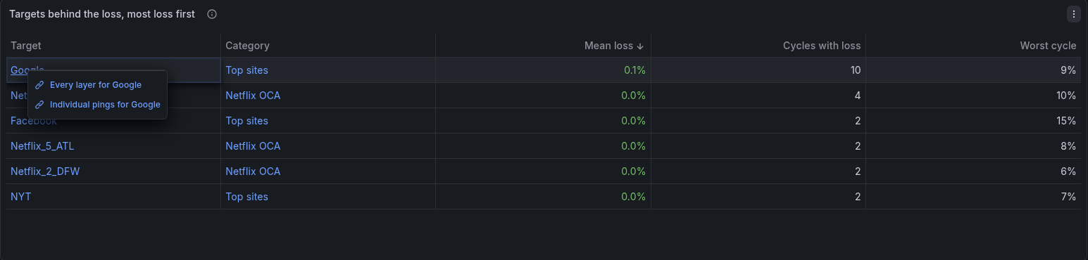
Targets behind the loss, most loss first lists every destination that lost packets in the selected range: the share of its pings lost, the number of probe cycles in which it lost at least one, and its worst cycle. Several targets of one category at the top is that category's problem; the same share on every target, whatever its category, is the link. A target name opens Target Detail (every layer of it on one page) or its individual pings; a category opens the side-by-side. As in the tiles, the ISP gateway and the DNS wizard's targets are left out.

The targets behind the loss, with a target's two links open - On the side-by-side, each panel's link icon and each series open Target Detail for that target, keeping the range.

The links keep the time range you are looking at, so the burst you clicked on is still in view two dashboards later.

When does it happen?¶

The four heatmaps cover the last 30 days, whatever the range picker says. Each cell is one hour of one day in the dashboard's time zone (the browser's unless Grafana is set otherwise). A band at the same hour across the days is a daily pattern; a single bright cell is one event.

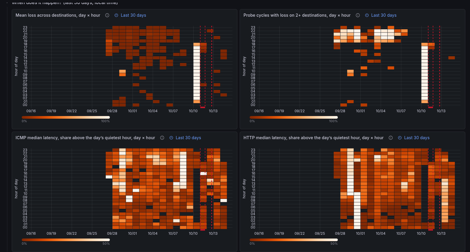
Loss and latency by day and hour of day, over 30 days

Mean loss across destinations. A single long cut lights a cell brightly. The color scale is compressed so that small everyday loss still shows.
Probe cycles with loss on 2+ destinations. The share of that hour's cycles in which destinations lost packets together. A cut counts once per cycle, however deep it was. A recurring evening band here is loss the destinations share, every day at the same time.
ICMP median latency, share above the day's quietest hour. The hourly mean of the median latency across destinations, as a share above the lowest hour of that same day. Latency moves by a few percent where loss moves by orders of magnitude, so an absolute scale would show nothing: relative to the day's own floor, a 19 ms and a 40 ms connection read alike, and the nightly rise that goes with the loss band shows. Each day's quietest hour is blank, and the scale saturates at +50 %. The first and the last day have fewer hours, and take their floor from those. A step between days (the whole connection getting slower) is not shown here; the latency chart above keeps it.
HTTP median latency, share above the day's quietest hour. The same, for the HTTP probes. HTTP time includes the servers' side, so a band here that the ICMP heatmap does not share is beyond the network: the sites, or the path to them, are slower at that hour.

A band in the heatmaps while the ISP gateway's loss line stays flat is beyond the access link. A band that appears together with Wi-Fi drops (see the Wi-Fi dashboard) is closer to home.

Two signals were tried and left out because the reference installation showed no daily band: the ISP gateway's loss (about two weeks of data; it lost pings only in the hours when every destination did, and outside those its hour-of-day mean never exceeded 0.4 %) and the Wi-Fi link's signal (30 days; its hourly mean moved by 0.6 dB across the 24 hours of the day).

Shading a window of your choice¶

Once the heatmaps show you a band, the Selected window box at the top of the dashboard shades it on every day of the selected range, on each time-axis panel, so you can see what loss, latency and the detected episodes did inside it. Type the window as HH:MM-HH:MM in the dashboard's time zone, for example 20:00-23:00; a window that crosses midnight, such as 23:00-02:00, works too. Leave the box empty, or type anything that is not two clock times, and nothing is shaded. On the day the clocks change, the window still follows the wall clock.

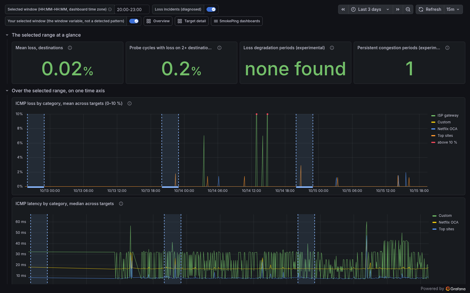
A selected window shaded on every day of the range

The shading is the annotation Your selected window (not a detected pattern), and its hover text repeats the window you typed. The name says what it is: a band you chose, generated from the variable, with no judgment behind it. The dashboard does not detect recurring windows by itself. If it ever did, the detected band would be a separate annotation set with its own name and color, never this one, so that what you selected and what the system found can never be read as the same thing. Whether to build that detection is an open decision, not a planned feature.